It is common to be a part of observe the following scenario:
- Data scientist spends several weeks in a Jupyter notebook
Actually, that’s not how it begins:
- Data scientist asks a data engineer where to find some neatly structured, accurately labelled data
- Data engineer says best I can do is [🍝 SQL query]
- Data scientist spends several weeks in a Jupyter notebook
- Some model metrics are paraded around, stakeholders are either happy or afraid to ask what on earth is a F1-score and what does car racing have to do with any of this
- An unholy union of data/platform/ML/backend engineers
sacrifice a product manager?deploy the model - No one bothers with the deployed model again. Yay, realised business value.

The Problem
The problem is one of entropy.
Then everything is; so let’s get a bit more specific.
Assume a model is 90% accurate. Without doing any extra work—i.e. no additional training—the performance of the model can
- Get better over time
- Stay the same
- Degrade over time
The first scenario is at odds with what we know about thermodynamics.
The second scenario is somewhat defensible, especially i) if you can tolerate some variation and ii) close your eyes and ears🙈🙉
The last scenario is real life.
For all intents and purposes, a learned machine learning model is at peak performance when it is first deployed (assuming you know what you are doing). If you don’t invest in additional follow-up work, you can safely assume your model performance will degrade over time at some point. Why? TL;DR: Things change IRL.
Why not re-train regularly? Labelled data is hard to come by and/or expensive. It’s hard to motivate stakeholders that this is a pressing issue. You may not have any monitoring in place at all. I’m glad I’m not speaking from experience.
An Elegant Solution
NannyML is an open-source post-deployment model monitoring (phew) framework in Python.
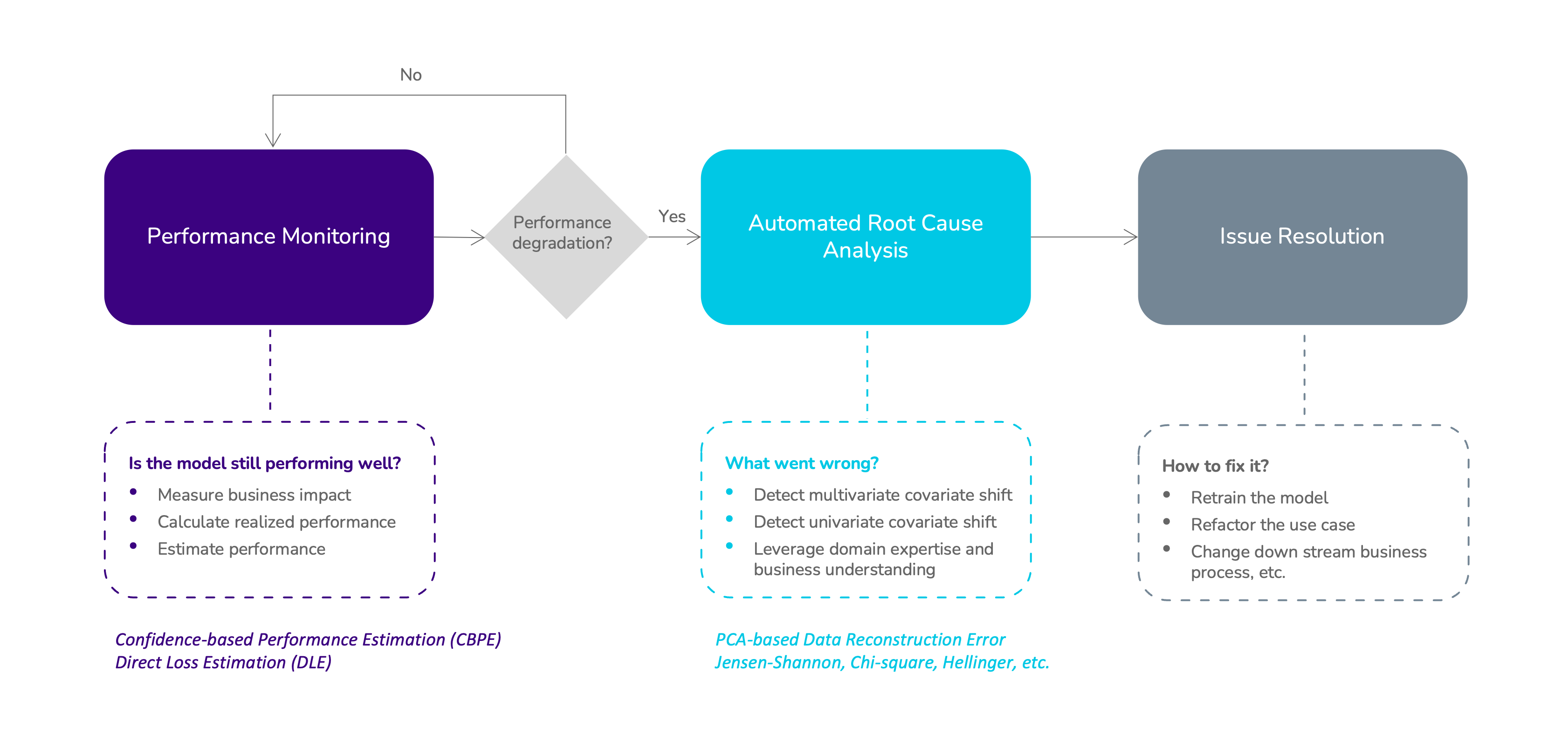
It comes packed with quite clever features, some of which do not rely on labelled data at all. Meaning, all the calculations are done on the features only—you must be capturing them if the model is in production—which is great news for us data practitioners.
| Data | Feature Drift | Output Drift | |
|---|---|---|---|
| Univariate | Multivariate | ||
| timestamp | |||
| features | X | X | |
| y_pred_proba | X | ||
| y_pred | X | ||
| y_true |
I’ll give them extra credit as well. Their solution is not novel in the sense that it is a recurrent theme at the data water-coolers all over the world: You know, it’s expensive to annotate production data, but we can always just compare the distributions of the features over time, right? And then, no one does it. It is mighty nice of them to put together a package that is simple to use.
How it works in a nutshell:
- Create ‘chunks’ of data (similar to folds in CV); these can be time-, size-, or number-based
- Compare the distributions of the features across chunks using the usual suspects (e.g. Kolmogorov-Smirnov, earth mover’s distance) to detect univariate drift
- For more advanced cases (i.e. multivariate drift), compare the PCA data reconstruction error across chunks
The logic of the reconstruction error is as follows: PCA learns the internal structure of the data by reducing its dimension (i.e. the principal components). If there is no drift, the components should be mostly stable across chunks—not exactly, as PCA procedure incurs some information loss, so some variation is to be expected.
Note that NannyML does a bunch of other things as well: model performance estimation, business value estimation, and data quality monitoring to name a few. However, I will limit my case to feature drift detection that does not require gathering labels in production. This means we cannot detect concept drift—whether the underlying relationship between features and the outcome has changed—as that requires labelled data.
Setup
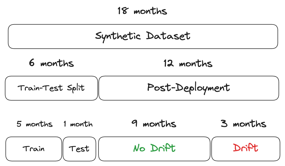
I will create some synthetic data so that we know what to look for. I will create data for 18 months, then split it—first 6 months for the train/test split, and the next 12 months for post-deployment monitoring. Every month consists of 1000 observations. I will manipulate some of the features in a way that they will drift after 9 months in production (i.e. something has changed IRL).
Let’s begin the setup with the imports and set the constants
import warnings
import nannyml as nml
import numpy as np
import pandas as pd

from sklearn.datasets import make_classification
from sklearn.ensemble import RandomForestClassifier
from sklearn.metrics import classification_report
from sklearn.model_selection import GridSearchCV, train_test_split
from sklearn.pipeline import Pipeline
from sklearn.preprocessing import StandardScaler

warnings.filterwarnings('ignore')

RANDOM_STATE = 1895
N_JOBS = -1
I generate 10 features, all of which are informative. I set the n_samples = 18000 to have 1000 observations per month. As all features are highly predictive, I will add some noise—i.e. make the classification task harder—by creating class imbalance weights and randomness flip_y
X, y = make_classification(n_features=10,
                           n_informative=10,
                           n_redundant=0,
                           n_repeated=0,
                           n_samples=18000,
                           weights=[0.7],
                           flip_y=0.25,
                           random_state=RANDOM_STATE)
This is how the data looks
X = pd.DataFrame(X)
X = X.add_prefix('feature_')
round(X.head(), 2)
## feature_0 feature_1 feature_2 ... feature_7 feature_8 feature_9
## 0 -0.10 1.19 1.05 ... 0.77 3.10 -3.22
## 1 2.64 4.31 2.01 ... -2.06 2.51 1.24
## 2 0.44 1.07 -0.33 ... 2.85 -0.83 -2.86
## 3 0.97 2.01 3.82 ... -2.94 2.07 1.85
## 4 2.00 -0.22 -0.27 ... -0.63 -0.99 0.67
##
## [5 rows x 10 columns]Next, I’ll quickly fit a random forest classifier to the data with some toy hyper-parameter search
pre_deployment = X.shape[0] // 3
X_train, X_test, y_train, y_test = train_test_split(X[:pre_deployment],
                                                    y[:pre_deployment],
                                                    train_size=0.8,
                                                    stratify=y[:pre_deployment],
                                                    random_state=RANDOM_STATE)
rf = Pipeline([('scaler', StandardScaler()),
               ('clf', RandomForestClassifier(n_jobs=N_JOBS,
                                              random_state=RANDOM_STATE))])
param_grid = {
    'clf__max_features': ['sqrt', 'log2'],
    'clf__bootstrap': [True, False]
}
gs = GridSearchCV(rf,
                  param_grid=param_grid,
                  cv=3,
                  scoring='roc_auc',
                  n_jobs=N_JOBS,
                  verbose=1)
gs.fit(X_train, y_train)
GridSearchCV(cv=3,
estimator=Pipeline(steps=[('scaler', StandardScaler()),
('clf',
RandomForestClassifier(n_jobs=-1,
random_state=1895))]),
n_jobs=-1,
param_grid={'clf__bootstrap': [True, False],
'clf__max_features': ['sqrt', 'log2']},
scoring='roc_auc', verbose=1)In a Jupyter environment, please rerun this cell to show the HTML representation or trust the notebook.On GitHub, the HTML representation is unable to render, please try loading this page with nbviewer.org.
GridSearchCV(cv=3,
             estimator=Pipeline(steps=[('scaler', StandardScaler()),
                                       ('clf',
                                        RandomForestClassifier(n_jobs=-1,
                                                               random_state=1895))]),
             n_jobs=-1,
             param_grid={'clf__bootstrap': [True, False],
                         'clf__max_features': ['sqrt', 'log2']},
scoring='roc_auc', verbose=1)Pipeline(steps=[('scaler', StandardScaler()),
('clf', RandomForestClassifier(n_jobs=-1, random_state=1895))])StandardScaler()
RandomForestClassifier(n_jobs=-1, random_state=1895)
preds = gs.predict(X_test)
print(classification_report(y_test, preds))
## precision recall f1-score support
##
## 0 0.83 0.95 0.89 789
## 1 0.87 0.64 0.73 411
##
## accuracy 0.84 1200
## macro avg 0.85 0.79 0.81 1200
## weighted avg 0.85 0.84 0.84 1200NannyML needs reference and analysis periods to detect drift. I will also add predicted labels and probabilities so that we can check for prediction drift as well.
I will create a post_deployment_df, which will contain the next 12 months of data after model training
y_predict_proba = gs.predict_proba(X[pre_deployment:])[:,0]
y_pred = gs.predict(X[pre_deployment:])
y_arrays = np.column_stack([y_predict_proba, y_pred])
post_deployment_df = pd.concat([
    X[pre_deployment:].reset_index(drop=True),
    pd.DataFrame(y_arrays, columns=['y_predict_proba', 'y_pred']),
], axis=1)
post_deployment_df['y_pred'] = np.where(post_deployment_df['y_pred'] == 0, 'No', 'Yes')
round(post_deployment_df.head(), 2)
## feature_0 feature_1 feature_2 ... feature_9 y_predict_proba y_pred
## 0 1.91 0.84 -0.24 ... -2.26 0.64 No
## 1 -1.96 5.20 5.28 ... -1.97 0.80 No
## 2 0.80 0.75 1.64 ... -1.10 0.92 No
## 3 4.30 0.50 0.68 ... 2.98 0.83 No
## 4 0.08 1.04 2.73 ... 2.73 0.24 Yes
##
## [5 rows x 12 columns]Adding timestamps will allow chunking and plotting easier
timestamp = np.repeat(pd.date_range(start='01-01-2022',
                                    periods=12,
                                    freq='M'),
                      1000)
post_deployment_df['timestamp'] = timestamp
Now, I will add progressive drift in the shape of Gaussian noise to two features—feature_4 and feature_7. The drift will begin 9 months into deployment and will get worse with each passing month, dictated by incrementing the standard deviation of the added noise
drifting_features = ['feature_4', 'feature_7']
for feature in drifting_features:
    for scale, timestamp in enumerate(pd.date_range(start='10-01-2022', periods=3, freq='M')):
        post_deployment_df.loc[post_deployment_df['timestamp'] == timestamp, feature] += np.random.normal(1, scale, 1000)
Finally, I will split the post_deployment_df into reference and analysis periods, lasting 9 months and 3 months, respectively
drift_cutoff = post_deployment_df['timestamp'] < '2022-10-01'
reference = post_deployment_df[drift_cutoff]
analysis = post_deployment_df.loc[~drift_cutoff]
Univariate Drift
NannyML can check whether a feature distribution has shifted between reference and analysis periods. For brevity, I will only use the Jensen-Shannon distance as the sole drift detection method. I will split the data into monthly chunks, which will raise a warning—three chunks is less than ideal and NannyML complains (suppressed in this notebook)
features = [col for col in reference.columns if 'feature' in col]
method = ['jensen_shannon']
uni_drift = nml.UnivariateDriftCalculator(
    column_names=features + ['y_pred'],
    timestamp_column_name='timestamp',
    continuous_methods=method,
    chunk_period='M'
)
uni_drift.fit(reference)
## <nannyml.drift.univariate.calculator.UnivariateDriftCalculator object at 0x2cb3f8710>uni_drift_results = uni_drift.calculate(analysis)Now that the calculations are done, we can plot the results. To set a baseline, let’s look at a stable feature first
figure = uni_drift_results.filter(column_names=['feature_0'],
                                  methods=method).plot(kind='drift')
figure.show()
And now, let’s plot the drifting features
figure = uni_drift_results.filter(column_names=drifting_features,
                                  methods=method).plot(kind='drift')
figure.show()
We can also plot the feature distributions over chunks, which can be a bit more intuitive
figure = uni_drift_results.filter(column_names=drifting_features,
                                  methods=method).plot(kind='distribution')
figure.show()
Nice. In both plots, we clearly see the drift starting in October and getting worse as time goes on.
Output Drift
Note that we can include the predicted labels—y_pred—when we called UnivariateDriftCalculator(). Similar to how we handled features, we can also check whether there is a shift in the distribution of predicted classes over time
figure = uni_drift_results.filter(column_names='y_pred',
                                  methods=method).plot(kind='distribution')
figure.show()
Despite feature drift in two predictors, the distribution of predicted classes is stable. Indeed, this can be collaborated with the number of alerts raised
alert_count_ranker = nml.AlertCountRanker()
alert_count_ranked_features = alert_count_ranker.rank(uni_drift_results)
alert_count_ranked_features.head()
## number_of_alerts column_name rank
## 0 3 feature_7 1
## 1 3 feature_4 2
## 2 0 y_pred 3
## 3 0 feature_9 4
## 4 0 feature_8 5Multivariate Drift
NannyML can also check whether there is an overall shift in the feature distributions, which collaborates the univariate results
multi_drift = nml.DataReconstructionDriftCalculator(
    column_names=features,
    timestamp_column_name='timestamp',
    chunk_period='M'
)
multi_drift.fit(reference)
## <nannyml.drift.multivariate.data_reconstruction.calculator.DataReconstructionDriftCalculator object at 0x2cb2cedd0>multi_drift_results = multi_drift.calculate(analysis)
figure = multi_drift_results.plot()
figure.show()I tried something cheeky—I included a PCA step in the model fitting pipeline to see if it would diminish the results, but they were stable 🤷🏻♂️
Comparison with Random Forest Feature Importance
Damien Benveniste recently posted on LI a neat trick to detect drift. We used to do a similar procedure back in the day, but I will give him the credit following the rule of more influential gets the cake.
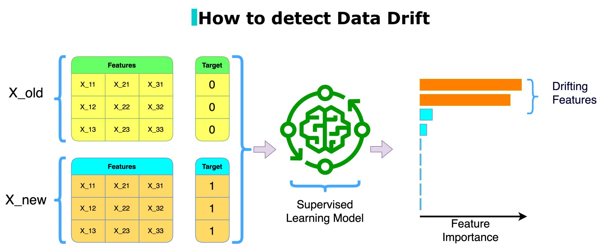
The trick is the following:
- Gather the features that are used by a production model in a dataset
- [Optional] To make the next step easier, add a date column
- Create a dummy indicator for the old/new data; say 0 for the last month’s records and 1 for the current month
- Fit a classifier that comes with built-in feature importance using the dummy indicator as the target
- If anything comes up as highly predictive, those features have drifted
post_deployment_df['drift'] = np.where(post_deployment_df['timestamp'] < '2022-10-01', 0, 1)
X_train, X_test, y_train, y_test = train_test_split(post_deployment_df.filter(regex='feature'), post_deployment_df['drift'],
                                                    stratify=post_deployment_df['drift'],
                                                    random_state=RANDOM_STATE)
rf = RandomForestClassifier(random_state=RANDOM_STATE)
rf.fit(X_train, y_train)RandomForestClassifier(random_state=1895)In a Jupyter environment, please rerun this cell to show the HTML representation or trust the notebook.
On GitHub, the HTML representation is unable to render, please try loading this page with nbviewer.org.
RandomForestClassifier(random_state=1895)
importances = pd.Series(rf.feature_importances_,
                        index=[i.replace('feature', 'ft') for i in rf.feature_names_in_])
importances.plot.bar()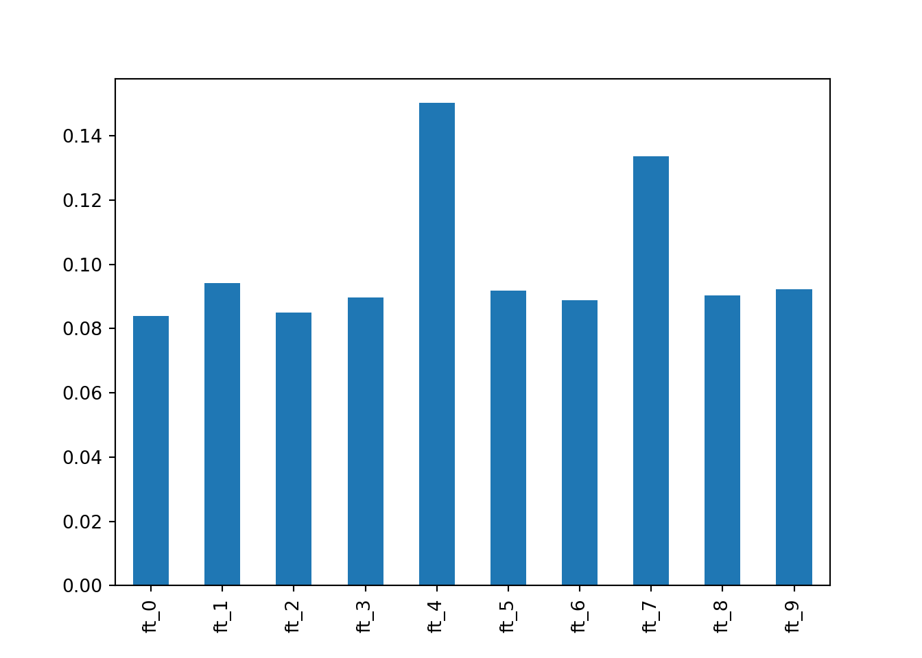
Yup, 4 and 7 be driftin’
Conclusion
NannyML is a great tool to detect drift in production models. When things are this intuitive and open-source, at the risk of sounding dramatic—you got a responsibility to use them. Don’t diminish the business value of your production models because you can’t be bothered!