A Tidytext Analysis of the Weinstein Effect

Quantifying He-Said, She-Said: Newspaper Reporting

I have been meaning to get into quantitative text analysis for a while. I initially planned this post to feature a different package (that I wanted to showcase), however I ran into some problems with their .json parsing methods and currently waiting for the issue to be solved on their end. The great thing about doing data science with R is that there are multiple avenues leading you to the same destination, so let’s take advantage of that.

My initial inspiration came from David Robinson’s post on gendered verbs. I remember sending it around and thinking it was quite cool. Turns out he was building on Julia Silge’s earlier post on gender pronouns. I see that post and I go, ‘what a gorgeous looking ggplot theme!’. So. Neat. Praise be the open source gods, the code is on GitHub. Let’s take advantage of that too.

I still needed a topic, and even though both the Wikipedia plots and the Jane Austen datasets sound interesting to look at, I felt that there is another, obvious choice.¹ It has a Wikipedia page and its own subreddit. Also, the title might have given it away. Let’s get to work.

Getting Full Text News Articles

My first instinct was to check out the NYT APIs—it made sense, given that they broke the news (along with the New Yorker). Everything seemed to be working out just fine, until I realised you cannot get the full text—only the lead. Staying true to my strict data scientist training, I googled ‘full text newspaper api r’ and there it was: GuardianR. Sorry NYC mates, we reckon we will have to cross the pond for this one.

Note that any one source will always be biased. If you are not familiar with the Guardian, it’s British and has a left-centre bias. It might be prudent to pair it with a right-centre newspaper, however not all newspapers provide APIs (which in itself is another selection bias). Alas, we will move on just with the Guardian—insert idiom regarding salt. Finally, you will need to get a free API key from their open source platform. You still have to register, but you are only in danger if you vote Tory and stand on the left side of the escalator. Once you got it, install/load the package via CRAN:

library(GuardianR)
ls(pos = "package:GuardianR")

## [1] "get_guardian"     "get_json"         "parse_json_to_df"

As you can see, the GuardianR package is a simple one: it contains only three (but powerful) functions. We only need the first one to get a hold of the full text articles, and the syntax is super simple:

#not evaluated
articles <- get_guardian(keywords = "sexual+harassment",
                         section = "world",
                         from.date = "2012-11-30",
                         to.date = "2017-11-30",
                         api.key = "your-key-here")

Running the above chunk with your own key will get you all articles published in the Guardian in the last five years tagged under the news section ‘world’² and containing the keywords ‘sexual harassment’ in the Guardian API. The keywords can be as simple or complicated as you want; just add more terms using the plus sign.

You might think the time frame is a bit skewed towards the ‘pre’ era—the news broke out on October 5, 2017. Going all the way back five full years, we are comparing 58 months worth of ‘pre’ to only 2 months of ‘post’ Weinstein. However, luckily for you blog posts are not written in real-time, meaning you get to see a (somewhat working) final result so just bear with me. And no, this is not at all like scientists running 514 regressions and failing to mention this tidbit in their publication. Relevant xkcd.

No, the reason is pure pragmatism. It’s not that running the code ‘live’ and getting the articles ‘real-time’ would not slow down this page—it’s not how it works.³ However, it is good practice to extract a tad bigger chunk than you think you will need, as you can always slice it up later to suit your needs better.

In any case, I am working with downloaded data so I will just load it up. Feel free to subset the data to see whether the results change if you use a different cut-off point. Also, if you go back the same amount of time (i.e. two months before October 5), that would lead to 183 articles for pre and 121 articles for the post time period—it is a reckoning, alright. Going back five years gets us 1224 articles in total; so we actually have 1103-pre and 121-post articles (89% to 11%). That’s more or less cross-validation ratio (well, a bit on the less side maybe), and we will roll with that for now.

articles <- read.csv("articles.csv", stringsAsFactors = FALSE)
dim(articles)

## [1] 1224   27

sum(articles$wordcount)

## [1] 1352717

colnames(articles)

##  [1] "id"                   "sectionId"            "sectionName"         
##  [4] "webPublicationDate"   "webTitle"             "webUrl"              
##  [7] "apiUrl"               "newspaperPageNumber"  "trailText"           
## [10] "headline"             "showInRelatedContent" "lastModified"        
## [13] "hasStoryPackage"      "score"                "standfirst"          
## [16] "shortUrl"             "wordcount"            "commentable"         
## [19] "allowUgc"             "isPremoderated"       "byline"              
## [22] "publication"          "newspaperEditionDate" "shouldHideAdverts"   
## [25] "liveBloggingNow"      "commentCloseDate"     "body"

We get a bunch of variables (27) with that call, but we won’t be needing most of them for our analysis:

#laziest subset for only two variables
want.var <- c("webPublicationDate", "body")
want <- which(colnames(articles) %in% want.var)
articles <- articles[, want]
articles$webPublicationDate <- as.Date.factor(articles$webPublicationDate)

The body contains the full-text, however it’s in HTML:

dplyr::glimpse(articles$body[1])

##  chr "<p>Numerous women have accused Don Burke of indecent assault, sexual harassment and bullying during the 1980s a"| __truncated__

At this point, I must admit I resorted to hacking a bit. I’m sure there is a more elegant solution here. I’ll go with this SO answer to extract text from HTML. Basically, the cleaning function removes the HTML using regex. Unfortunately, this does not clear up various apostrophes found in the text. For that, we switch the encoding from ASCII to byte:

articles$body <- iconv(articles$body, "", "ASCII", "byte")

cleanFun <- function(htmlString) {
  return(gsub("<.*?>", "", htmlString))
}

articles$body <- cleanFun(articles$body)
dplyr::glimpse(articles$body[1])

##  chr "Numerous women have accused Don Burke of indecent assault, sexual harassment and bullying during the 1980s and "| __truncated__

This will end up cutting some legitimate apostrophes (e.g. “hasn’t”, “didn’t” to “hasn”, “didn”) in some cases, but we will fix that later on.

Let’s split the data on date October 5, 2017 and get rid of the date column afterwards:

#You can also use negative index for subsetting
articles.before <- articles[articles$webPublicationDate < "2017-10-05", ]
articles.after <- articles[articles$webPublicationDate >= "2017-10-05", ]

full.text.before <- articles.before[, 2]
full.text.before <- as.data.frame(full.text.before)

full.text.after <- articles.after[, 2]
full.text.after <- as.data.frame(full.text.after)

N-Grams and Combinatorics

To me, n-grams are what prisoner’s dilemma to college freshman—that ‘wow, so simple but so cool’ moment. As in, simple after the fact when someone has already figured it out and explained it to you. N-grams are essentially combinations of n words. For example, a bigram (2-gram).⁴ Using the tidytext package developed by David and Julia, we can create them in a flash with unnest_tokens. After that, we will separate the bigrams into two distinct words. Next, we will subset the bigrams so that the first word is either he or she. Finally, we will transform the words into frequency counts. I’m heavily recycling their code—no need to reinvent the wheel:

library(tidytext)
library(tidyverse) #or just dplyr and tidyr if you are allergic

#Create bigrams
bigrams.before <- full.text.before %>%
  unnest_tokens(bigram,
                full.text.before,
                token = "ngrams",
                n = 2)
nrow(bigrams.before)

## [1] 1311051

head(bigrams.before)

##        bigram
## 1    the walk
## 1.1 walk from
## 1.2  from the
## 1.3  the gare
## 1.4   gare du
## 1.5   du nord

#Separate bigrams into two words
bigrams.separated.before <- bigrams.before %>%
  separate(bigram, c("word1", "word2"), sep = " ")

head(bigrams.separated.before)

##     word1 word2
## 1     the  walk
## 1.1  walk  from
## 1.2  from   the
## 1.3   the  gare
## 1.4  gare    du
## 1.5    du  nord

#Subset he and she in word1
he.she.words.before <- bigrams.separated.before %>%
  filter(word1 %in% c("he", "she"))

#Fix the missing t's after apostrophe
fix.apos <- c("hasn", "hadn", "doesn", "didn", "isn", "wasn", "couldn", "wouldn")
he.she.words.before <- he.she.words.before %>%
  mutate(word2 = ifelse(word2 %in% fix.apos, paste0(word2, "t"), word2))
  
#10 random samples; the numbers are row numbers not counts
set.seed(1895)
dplyr::sample_n(he.she.words.before, 10)

##       word1  word2
## 4403    she doesnt
## 3732     he    was
## 5222    she  wasnt
## 11862   she   said
## 3972    she  wrote
## 3189     he   says
## 3952    she   sees
## 4878     he    was
## 9314     he   went
## 9408    she  noted

#Transform words into counts, add +1 for log transformation
he.she.counts.before <- he.she.words.before %>%
  count(word1, word2) %>%
  spread(word1, n, fill = 0) %>%
  mutate(total = he + she,
         he = (he + 1) / sum(he + 1),
         she = (she + 1) / sum(she + 1),
         log.ratio = log2(she / he),
         abs.ratio = abs(log.ratio)) %>%
  arrange(desc(log.ratio))

#Top 5 words after she
head(he.she.counts.before)

## # A tibble: 6 x 6
##       word2           he          she total log.ratio abs.ratio
##       <chr>        <dbl>        <dbl> <dbl>     <dbl>     <dbl>
## 1 testified 0.0002194908 0.0027206771    18  3.631734  3.631734
## 2     awoke 0.0001097454 0.0010580411     6  3.269163  3.269163
## 3     filed 0.0002194908 0.0021160822    14  3.269163  3.269163
## 4      woke 0.0002194908 0.0019649335    13  3.162248  3.162248
## 5    misses 0.0001097454 0.0007557437     4  2.783737  2.783737
## 6   quickly 0.0001097454 0.0007557437     4  2.783737  2.783737

A couple of observations. First, n-grams overlap, resulting in 1.6M observations (and this is only the pre-period). However, we will only use the gendered subset,⁵ which is much more smaller in size. Second, as we define the log ratio as (she / he), the sign of the log ratio determines the direction (positive for she, negative for he), while the absolute value of the log ratio is just the effect size (without direction).

Good stuff, no? Wait until you see the visualisations.

Let There Be GGraphs

Both David and Julia utilise neat data visualisations to drive home their point. I especially like the roboto theme/font, so I will just go ahead and use it. You need to install the fonts separately, so if you are missing them you will get an error message.

devtools::install_github("juliasilge/silgelib")
#Required Fonts
#https://fonts.google.com/specimen/Roboto+Condensed
#https://fonts.google.com/specimen/Roboto
library(ggplot2)
library(ggrepel)
library(scales)
library(silgelib) 
theme_set(theme_roboto())

We are also loading several other libraries.⁶ In addition to the usual suspects, ggrepel will make sure we can plot overlapping labels in a bit nicer way. Let’s start by looking at the most gendered verbs in articles on sexual harassment. In other words, we are identifying which verbs are most skewed towards one gender. I maintain the original logarithmic scale, so the effect sizes are in magnitudes and easy to interpret. If you read the blog posts, you will notice that Julia reports a unidirectional magnitude (relative to she/he), so her scales go from

.25x .5x x 2x 4x

whereas David uses directions, i.e.

'more he' 4x 2x x 2x 4x 'more she'

In both cases, x denotes the same frequency (equally likely) of usage. I don’t think one approach is necessarily better than the other, but I went with David’s approach. Finally, I filter out non-verbs plus ‘have’ and only plot verbs that occur at least five times. If you are serious about filtering out (or the opposite, filtering on) classes of words—say a certain sentiment or a set of adjectives—you should locate a dictionary from an NLP package and extract the relevant words from there. Here, I am doing it quite ad-hoc (and manually):

he.she.counts.before %>%
  filter(!word2 %in% c("himself", "herself", "ever", "quickly",
                       "actually", "sexually", "allegedly", "have"),
         total >= 5) %>%
  group_by(direction = ifelse(log.ratio > 0, 'More "she"', "More 'he'")) %>%
  top_n(15, abs.ratio) %>%
  ungroup() %>%
  mutate(word2 = reorder(word2, log.ratio)) %>%
  ggplot(aes(word2, log.ratio, fill = direction)) +
  geom_col() +
  coord_flip() +
  labs(x = "",
       y = 'Relative appearance after "she" compared to "he"',
       fill = "",
       title = "Pre Weinstein: 2012-17 The Guardian Articles on Sexual Harassment",
       subtitle = "Top 15 Most Gendered (Skewed) Verbs after he/she; at least 5 occurrences.") +
  scale_y_continuous(labels = c("8X", "6X", "4X", "2X", "Same", "2X", "4X", "6X", "8X"),
                     breaks = seq(-4, 4)) +
  guides(fill = guide_legend(reverse = TRUE)) +
  expand_limits(y = c(-4, 4))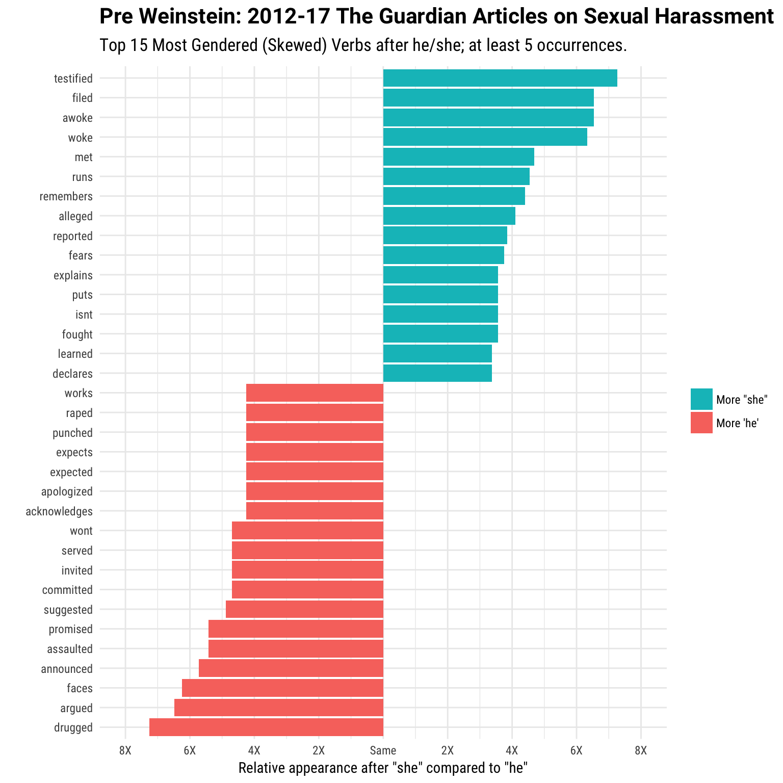

Several immediate and depressing trends emerge from the data. The top active verbs for women cluster on bringing charges: ‘testified’, ‘filed’; whereas male verbs seem to react to those with ‘argued’, ‘faces’, ‘acknowledges’, and ‘apologized’. Women ‘awoke’ and ‘woke’, matching the more violent male verbs such as ‘drugged’, ‘assaulted’, ‘punched’, and ‘raped’. ‘Alleged’ occurs four times more after she relative to he, and there is no mention of denial (e.g. ‘denied’, ‘denies’) after he. A note on word variations: in some cases, it might be better to combine conjugations into a single category using a wildcard (such as expect* in the graph above). However, I thought the tense can also contribute to a quantitative story, so I left them as they are.

Another way of visualising the gendered differences is to plot their magnitude in addition to their frequency. This time, we are not limited to just verbs; however we still filter out some uninteresting words. There are additional ggplot and ggrepel arguments in this plot. First, I added two reference lines: a red y-intercept with geom_hline to act as a baseline and an invisible x-intercept using geom_vline to give the labels more space on the left-hand side. Do you not love tidy grammar? Last but not least, I insert geom_text_repel to give us more readability: segment.alpha controls the line transparency, while the force argument governs the aggressiveness of the jittering algorithm. We could supply it with a fill argument that corresponds to a factor variable to highlight a certain characteristic (say, total occurrence), however there is not much meaningful variation there in our case.

he.she.counts.before %>%
  filter(!word2 %in% c("himself", "herself", "she", "too", "later", "apos", "just", "says"),
         total >= 10) %>%
  top_n(100, abs.ratio) %>%
  ggplot(aes(total, log.ratio)) +
  geom_point() +
  geom_vline(xintercept = 5, color = "NA") +
  geom_hline(yintercept = 0, color = "red") +
  scale_x_log10(breaks = c(10, 100, 1000)) +
  geom_text_repel(aes(label = word2), segment.alpha = .1, force = 2) +
  scale_y_continuous(breaks = seq(-4, 4),
                     labels = c('8X "he"', '6X "he"', '4X "he"', '2X "he"', "Same",
                                '2X "she"', '4X "she"', '6X "she"', '8X "she"')) +
  labs(x = 'Total uses after "he" or "she" (Logarithmic scale)',
       y = 'Relative uses after "she" to after "he"',
       title = "Gendered Reporting: Pre Weinstein, The Guardian",
       subtitle = "Words occurring at least 10 times after he/she:
                  160 unique words (100 displayed) | 11,013 occurrences in total") +
  expand_limits(y = c(4, -4))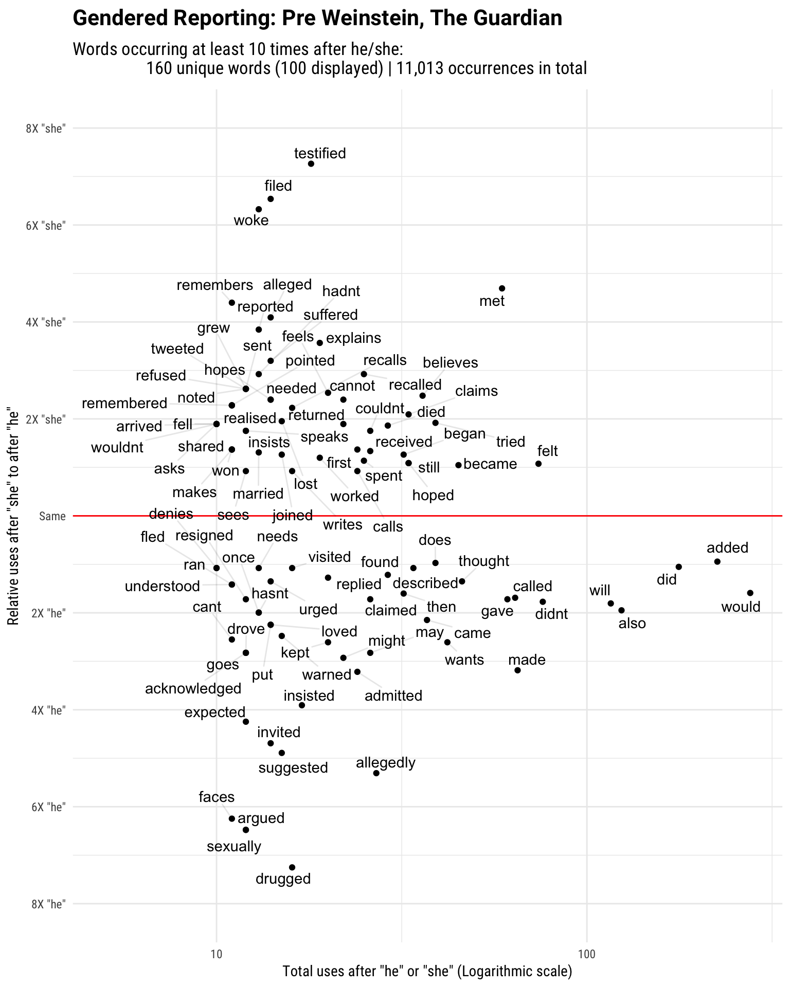

Plotting frequencies complement the first plot quite nicely. We can infer reported characteristics more easily when there is a tangible baseline. Words around the red line occur after she or he more or less equally: the y-axis determines the relational effect size (with regards to gender), and the x-axis displays the total amount of occurrences. Some additional insights: we see that ‘sexually’ and ‘allegedly’ popping up after he quite frequently. There is also the verb ‘admitted’, as well as ‘denies’ (even though visually it is located above the red line, if you follow the grey segment, it’s located around 1X ‘he’). For women, more morbid words like ‘suffered’, ‘died’ are added to the mix. There are also nuances regarding the tense; ‘claims’ follows she twice more than he, while ‘claimed’ is twice likely to come after he.⁷

Moving on to the post-Weinstein period (‘the effect’), I quietly run the same code, and plot the equivalent graphics below. Some caveats: with the smaller sample size, I lowered the inclusion threshold from 5 to 2. Additionally, although it is top 15 most skewed verbs per gender, because of frequent ties, it ends up having more than that at the end.

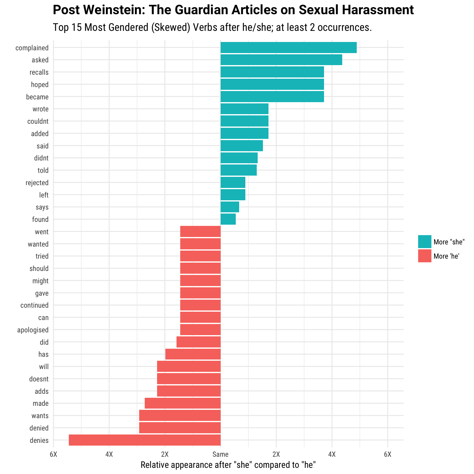
After the scandal broke, we see that women are reported to have ‘complained’, ‘hoped’, and ‘became’. On the other hand, men are vehemently denying the accusations, with ‘denies’ and ‘denied’ being the most skewed verbs following he. Random point: in the pre-period, it’s ‘apologized’, in the post-period, it’s ‘apologised’. Maybe Brexit can manifest in mysterious ways.

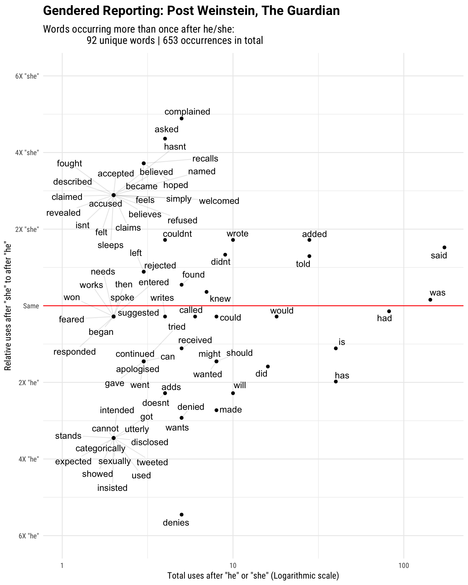
Again we turn to the frequency plot to infer more. In addition to denial, men are also reported to use words such as ‘categorically’ and ‘utterly’. Both ‘claims’ and ‘claimed’ occur more after she, not repeating the earlier dynamic regarding the tense. In addition, we don’t see ‘alleged’ or ‘allegedly’ featured in the plot at all. How much of this change can we attribute to the effect? At a glance, we definitely see a difference. For example, verbs display a good variation for both genders. The post-frequency plot features less violent words than the pre-frequency plot. There is a lot more ‘denying’ and not much ‘alleging’ in the post-Weinstein period.

Some are definitely data artefacts. The post-frequency plot is ‘cleaner’—in addition to (and directly caused by) the smaller n—because the cut-off point is set to ‘more than once’: if we remove the filter, all the violence and harassment terms are back in. Some are probably reporter/reporting biases plus the prevalent gendered thinking (that occurs both on a conscious level and below). And perhaps some are genuine effects—true signal. It is still too early to pass judgement on whether the Weinstein effect will result in tangible, positive change. Currently, all we can get is a short, limited glimpse at the available data.

Hopefully you managed to enjoy this rather depressing data undertaking using the tidytext package. As usual, the underlying code is available on GitHub. N-grams are powerful. Imagine the possibilities: assume you have access to a rich dataset (say, minimum 100K very long articles/essays). You can construct n-grams sequentially; i.e. 2-grams; 3-grams, 4-grams etc., separate the words, and subset for gendered pronouns. This would give you access to structures like “he” + “word” + “her” (direct action) and “she” + “word” + “word” + “him” (allowing for adjective + verb). Then it would be possible to look for all kinds of interactions, revealing their underlying structure. I will be reporting more on this front, until I move onto image processing (looking at you, keras).