Dealing with Correlated High-Dimensional Data

Theory to Application ¹

I recently realized my review of Michael Alvarez’s edited volume Computational Social Science: Discovery and Prediction went online a while ago. If memory serves, used to be the case that book reviews were freely available; alas now even a 400-word long piece is behind a paywall. I initially planned to do a post covering the whole book—at least the application part, as the volume is neatly segregated on theory vs. application lines. And instead of going through various applied tools, which is what the edited volume successfully accomplishes, I decided to pick a particular method and give it a test drive. Disclaimer—the example would not necessarily pass as a social science enterprise, but the data challenge it poses makes it relevant for all type of users.

Fuzzy forests, in addition to being situated on the better side of the statistical method naming spectrum (don’t you just want to use them?), advertises a neat improvement over the regular randomForest package in R—the ability to deal with correlated, high dimensional data. Cast in the fiery realms of biostats, the algorithm relies on Weighted Gene Coexpression Network Analysis (WGCNA) to create uncorrelated sets of features called modules. These modules in turn are separately fed to recursive feature elimination random forests (RFE-RFs). The ‘surviving’ features—the ones that made it to the last round—go through a final round of RFE-RFs. At this point, based on a user-specified length of a ranked variable importance list (more on that in a bit), the selected features can be used to train a predictive model.

Given this high dimensional premise, let’s compare the vanilla random forest algorithm to the fuzzy forest. If fuzzy forests sound like fitting a random forest after doing a principal component analysis, you are not alone. However, this inevitably invites questions about interpretability: Random forests get enough flak for being black boxes, and now we are adding extra mathemagic by introducing loadings. One might argue it is better to stick with regular random forests if the marginal utility of making them ‘fuzzy’ does not pay off.

The standard way of comparing these two algorithms would be simply to evalute the predictive ability of both in the presence of high dimensional data. However, this is more or less the point of the introductory paper linked earlier. Let’s consider the interpretability and stability of the results instead. Do the algorithms generate convergent or divergent insights? Fuzzy forests require preprocessing—is it worth the trouble if one can get equivalent results from RFs out of the box? Let’s find out.

Data Setup

fuzzyforest comes prepackaged with a dataset on gene expression levels in liver tissue. The attached subset has 66 observations (female mice) and 3600 variables (gene expression measurements); the good old 1:600 ratio of p to n. The first variable in the dataset is weight (g), which I will treat as the outcome we want to predict. Unsurprisingly, its a continuous variable. Later, given 1:600 p to n ratio is not serious enough of a handicap with an n of 66, we will go ahead and shoot ourselves in the other foot (lose more data) by converting the outcome into a binary variable. Although this is probably a pretty terrible idea, this superficial constraint might shed light on the extent of the algorithm capabilities (i.e. robustness or its lack of) in our comparison.

library(fuzzyforest)
data(Liver_Expr)
dim(Liver_Expr) #yikes

## [1]   66 3601

weight <- Liver_Expr[, 1]
expression_levels <- Liver_Expr[, -1]
summary(weight)

##    Min. 1st Qu.  Median    Mean 3rd Qu.    Max. 
##   22.20   33.70   37.10   37.25   42.45   54.10

hist(weight) #look at that perfectly coincidental normal distribution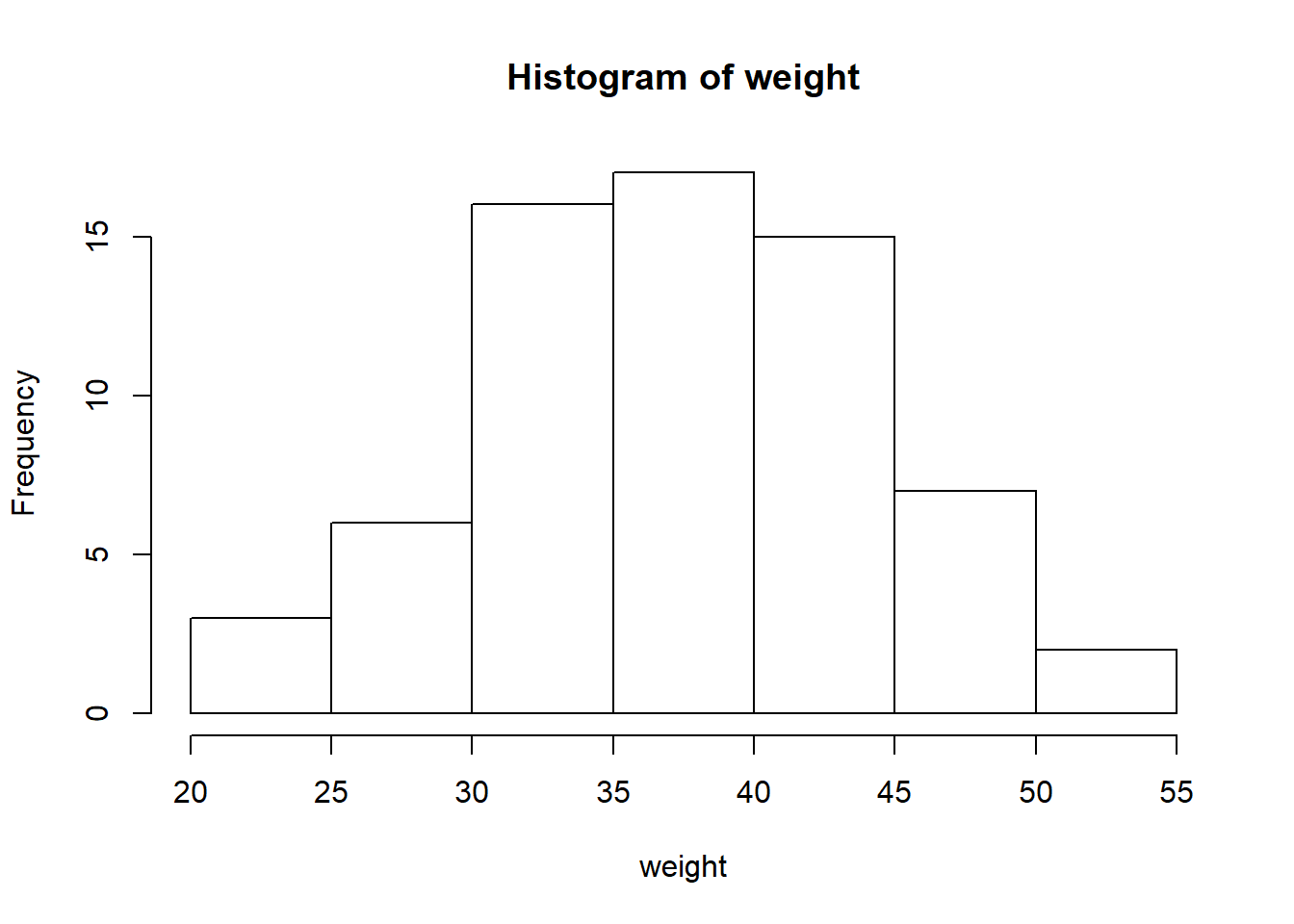

Random Forest

Let’s take a step back and try fitting a random forest without going through the WCGNA process. For the first pass, we will not bother tuning the parameters—we just want to obtain a ballpark OOB error rate to act as a baseline. Note that you can call tuneRF to get optimal ntree and mtry values.

library(randomForest)
set.seed(1895)
rf_fit <- randomForest(expression_levels, weight, ntree = 1000, importance = TRUE)
rf_fit

## 
## Call:
##  randomForest(x = expression_levels, y = weight, ntree = 1000,      importance = TRUE) 
##                Type of random forest: regression
##                      Number of trees: 1000
## No. of variables tried at each split: 1200
## 
##           Mean of squared residuals: 12.90961
##                     % Var explained: 71.92

varImpPlot(rf_fit, n.var = 10)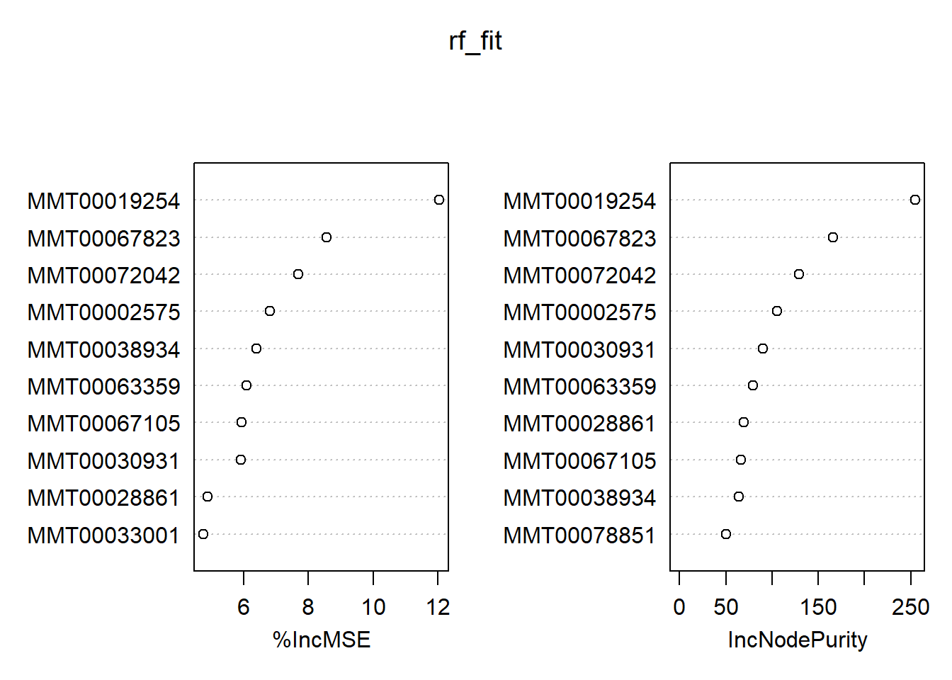

Even though we have 1000 trees for 3600 variables, the RF algorithm considers 1200(!) variables to choose from that pool for every decision for regression problems by default. Our casual model explains around 72% of the variance, and we plotted the top ten predictors based on their performance. If you are particularly lazy, you can extract them using the pdp package:

library(pdp)
topPredictors(rf_fit, n = 10)

##  [1] "MMT00019254" "MMT00067823" "MMT00072042" "MMT00002575" "MMT00038934"
##  [6] "MMT00063359" "MMT00067105" "MMT00030931" "MMT00028861" "MMT00033001"

This was for regression. Let’s have a quick glance at its classification variant:

Liver_Expr$weight_class <- ifelse(Liver_Expr$weight < mean(Liver_Expr$weight), 0, 1)
weight_class <- as.factor(Liver_Expr$weight_class)
rf_fit_cl <- randomForest(expression_levels, weight_class, ntree = 1000, importance = TRUE)
rf_fit_cl

## 
## Call:
##  randomForest(x = expression_levels, y = weight_class, ntree = 1000,      importance = TRUE) 
##                Type of random forest: classification
##                      Number of trees: 1000
## No. of variables tried at each split: 60
## 
##         OOB estimate of  error rate: 12.12%
## Confusion matrix:
##    0  1 class.error
## 0 32  3  0.08571429
## 1  5 26  0.16129032

varImpPlot(rf_fit_cl, n.var = 10)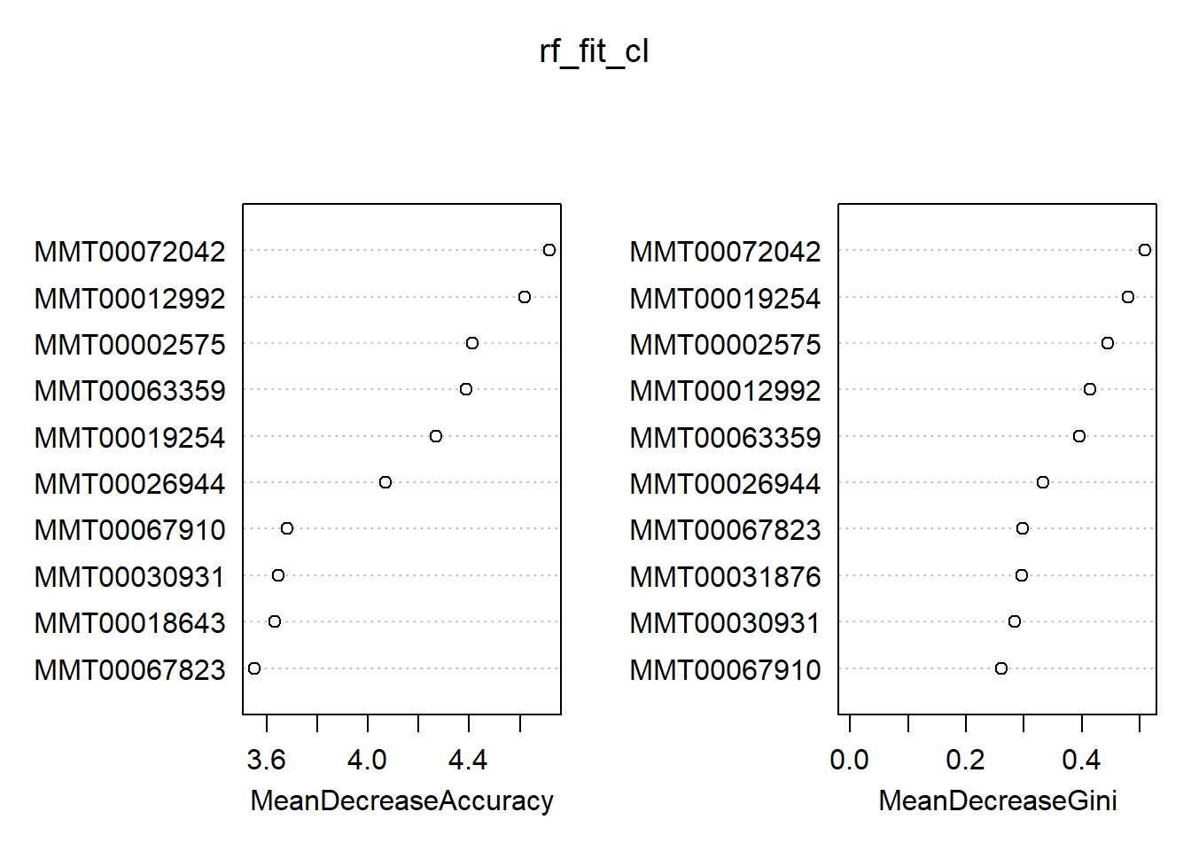

Out of the box, we get an OOB estimate of 12%. This time, the default choice of mtry is 60 (down from 1200 for the regression problem). We see a slight tendency for the ‘lighter’ class—the RF did a better job identifying the zeroes. In general, we find there is quite the overlap between the classification and regression results in terms of the top ten most important variables. However, this is not necessarily a smoking gun; the heavier weight class might have a slightly different set of characteristics compared to that of a continuum of weights. On a final note, you can generate a full report of your forest via the aptly named randomForestExplainer package. To illustrate, calling explain_forest(rf_fit) would result in this document. Definitely not a black box anymore!

Fuzzy Forest

As I mentioned earlier, fuzzyforest depends on WGCNA for dimension reduction—we cannot fit a model right away. Although it is on CRAN, at least one dependency is on Bioconducter. To install WGCNA, run:

source("http://bioconductor.org/biocLite.R")
biocLite(c("AnnotationDbi", "impute", "GO.db", "preprocessCore"))
install.packages("WGCNA")

After you load the library, you can follow the example code from the publication to fit the model quickly. Note that this is somewhat optimized; at least in comparison to the RF setup we have above.

WGCNA_params <- WGCNA_control(power = 6, 
                              TOMType = "unsigned", 
                              minModuleSize = 30,
                              numericLabels = TRUE, 
                              pamRespectsDendro = FALSE)
mtry_factor <- 1; drop_fraction <- .25; number_selected <- 10
keep_fraction <- .05; min_ntree <- 5000; ntree_factor <- 5
final_ntree <- 5000;
screen_params <- screen_control(drop_fraction = drop_fraction,
                                keep_fraction = keep_fraction,
                                min_ntree = min_ntree,
                                mtry_factor = mtry_factor,
                                ntree_factor = ntree_factor)
select_params <- select_control(drop_fraction = drop_fraction,
                                number_selected = number_selected,
                                min_ntree = min_ntree,
                                mtry_factor = mtry_factor,
                                ntree_factor = ntree_factor)

I will not pretend Rmarkdown can handle fitting 3600 variables on the fly for the wff_fit object (the page would have taken a while to load). Hence, the below code is not evaluated. When you run it, don’t forget to change the number of processors at the end depending on your setup. The WGCNA package will produce a warning with instructions if it detects a multi-core system but no parallel processing enabled.

wff_fit <- wff(expression_levels, weight,
               WGCNA_params = WGCNA_params,
               screen_params = screen_params,
               select_params = select_params,
               final_ntree = final_ntree,
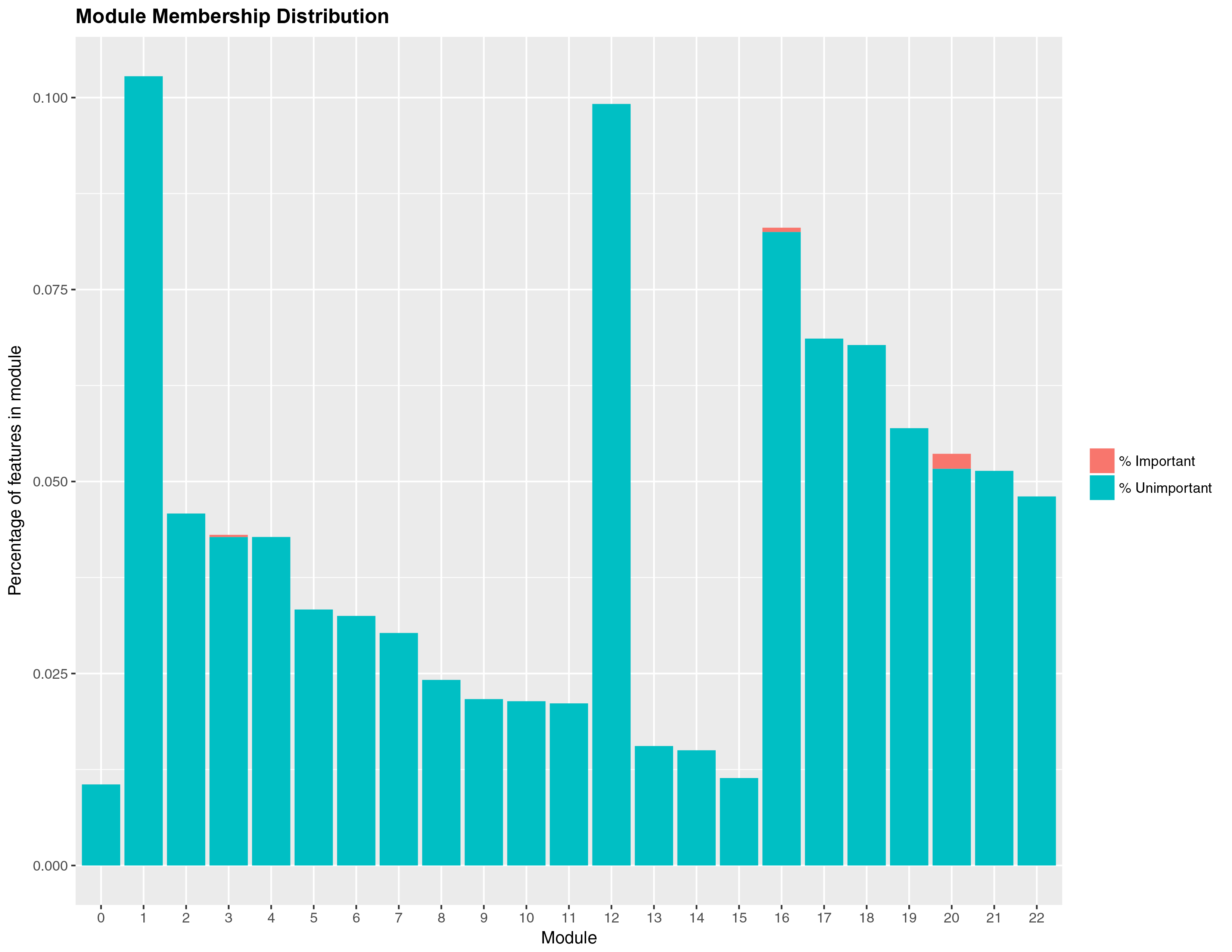
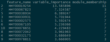
               num_processors = 8)

Once you are done fitting, you can access the results in several ways. You can get a list of the top predictors by calling print(wff_fit).² Finally, you can obtain a nice in-house graph plotting the module distribution by typing modplot(wff_fit). This gives us the relative importance of the modules. You should get something like the following:

And for the classification problem:

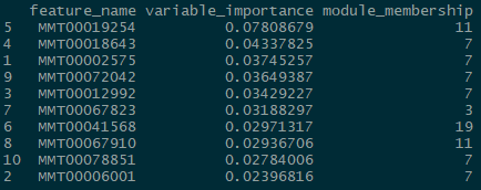
Again, somewhat similar variable selection, however here we see more variation. On the other hand, the similarities are quite striking when present: the top predictor (expression 19854) is the same, and modules 7 and 11 are the most influential ‘loadings’ for both types of problems.

If you are curious about how the fuzzy forest modules compare to PCA loadings, you can get an idea by setting the component number manually so that it matches the WGCNA process (22 in our example):

library(pcaMethods)
PCAmethods <- pca(Liver_Expr[, -1],
                  scale = "uv",
                  center = T,
                  nPcs = 22,
                  method = "svd")
print(PCAmethods)

## svd calculated PCA
## Importance of component(s):
##                  PC1    PC2    PC3     PC4     PC5    PC6     PC7     PC8
## R2            0.1883 0.1441 0.1215 0.06953 0.03955 0.0381 0.03553 0.03134
## Cumulative R2 0.1883 0.3323 0.4538 0.52332 0.56287 0.6010 0.63650 0.66784
##                   PC9    PC10    PC11    PC12    PC13    PC14    PC15
## R2            0.02848 0.02422 0.02009 0.01973 0.01678 0.01624 0.01533
## Cumulative R2 0.69632 0.72054 0.74063 0.76036 0.77714 0.79338 0.80871
##                  PC16   PC17   PC18    PC19    PC20    PC21    PC22
## R2            0.01403 0.0128 0.0124 0.01146 0.00974 0.00919 0.00865
## Cumulative R2 0.82274 0.8355 0.8479 0.85940 0.86914 0.87833 0.88698
## 3601     Variables
## 66   Samples
## 0    NAs ( 0 %)
## 22   Calculated component(s)
## Data was mean centered before running PCA 
## Data was scaled before running PCA 
## Scores structure:
## [1] 66 22
## Loadings structure:
## [1] 3601   22

We see that the increase in \(R^2\) begins to stagnate after the third component, a narrative we can corroborate with the FF modules for the regression problem (without making a claim about the makeup of the clusters). One can feed the loadings into a RF, however that will probably increase the difficulty level of your presentation if you actually need to convey your findings to a third-party. This is what it comes down to with FF as well.

Verdict? It’s a hard sell (for social science purposes).³ The performance of the RF—in terms of feature seletion—out of the box with no tuning looks like on par with what FF has to offer. Plus, FF requires preprocessing, either via WGCNA or prior knowledge, to work in the first place. The wide range of R packages that accept randomForest output is another decisive advantage. Don’t abandon the RF ship just yet.