Intro
Yesterday I gave a workshop on applied predictive modelling1 with caret at the 1st LSE Computational Social Science hackathon. Organiser privileges. I put together some introductory code and started a simple GitHub repo for the participants, so I thought I’d share it here as well. This is not supposed to cover all aspects of caret (plus there is already this), but more of a starter-pack for those who might be migrating from Python or another machine learning library like mlr. I have also saved the environment as caret.rdata, so that the participants can load it up during the workshop (insert harrowing experience about live coding) and follow through—that’s included in the repo too if you rather have a test run first.
The Data
Let’s start by creating some synthetic data using caret. The twoClassSim generates a dataset suitable for binary-outcomes:
dat <- twoClassSim(n = 1000, #number of rows
                   linearVars = 2, #linearly important variables
                   noiseVars = 5, #uncorrelated irrelevant variables
                   corrVars = 2, #correlated irrelevant variables
                   mislabel = .01) #percentage possibly mislabeled
colnames(dat)
## [1] "TwoFactor1" "TwoFactor2" "Linear1" "Linear2" "Nonlinear1"
## [6] "Nonlinear2" "Nonlinear3" "Noise1" "Noise2" "Noise3"
## [11] "Noise4" "Noise5" "Corr1" "Corr2" "Class"The above chunk simulates a dataframe with 1000 rows containing 15 variables:
- Class: Binary outcome (Class)
- TwoFactor: Correlated multivariate normal predictors (TwoFactor1, TwoFactor2)
- Nonlinear: Uncorrelated random uniform predictors (NonLinear1, …, Nonlinear3)
- Linear: (Optional) uncorrelated standard normal predictors (Linear1, Linear2)
- Noise: (Optional) uncorrelated standard normal predictors (Noise1, … , Noise5)
- Correlated: (Optional) correlated multivariate normal predictors (Corr1, Corr2)
We can take a closer look at the variables using two packages: skimr and xray. Both have functions that provide a snapshot of your covariates in an easy-to-understand output:
skim(dat) #unintended## Skim summary statistics
## n obs: 1000
## n variables: 15
##
## Variable type: factor
## variable missing complete n n_unique top_counts ordered
## Class 0 1000 1000 2 Cla: 567, Cla: 433, NA: 0 FALSE
##
## Variable type: numeric
## variable missing complete n mean sd p0 p25 median
## Corr1 0 1000 1000 -0.078 1 -3.19 -0.76 -0.11
## Corr2 0 1000 1000 -0.016 1 -2.91 -0.71 -0.014
## Linear1 0 1000 1000 0.016 1 -3.29 -0.68 0.054
## Linear2 0 1000 1000 0.023 1.02 -3.31 -0.66 0.053
## Noise1 0 1000 1000 -0.022 1 -3.46 -0.71 -0.023
## Noise2 0 1000 1000 -0.048 0.99 -3.52 -0.74 -0.042
## Noise3 0 1000 1000 0.016 0.97 -3.11 -0.64 0.014
## Noise4 0 1000 1000 -0.015 1.02 -3.48 -0.71 -0.028
## Noise5 0 1000 1000 0.036 0.94 -3.03 -0.59 0.072
## Nonlinear1 0 1000 1000 0.0086 0.58 -1 -0.49 0.038
## Nonlinear2 0 1000 1000 0.49 0.29 7.8e-05 0.25 0.5
## Nonlinear3 0 1000 1000 0.51 0.29 5e-04 0.26 0.52
## TwoFactor1 0 1000 1000 -0.086 1.36 -4.28 -0.96 -0.085
## TwoFactor2 0 1000 1000 -0.042 1.39 -4.63 -1.03 0.0095
## p75 p100 hist
## 0.58 3.58 ▁▂▆▇▇▂▁▁
## 0.67 3.57 ▁▂▅▇▆▂▁▁
## 0.71 3.02 ▁▁▃▇▇▅▂▁
## 0.69 3.88 ▁▂▅▇▇▂▁▁
## 0.64 3.22 ▁▁▃▇▇▅▁▁
## 0.61 3.39 ▁▁▅▇▇▅▁▁
## 0.64 3.77 ▁▁▅▇▅▂▁▁
## 0.67 3.17 ▁▁▃▇▇▅▁▁
## 0.71 3.1 ▁▁▅▇▇▅▁▁
## 0.5 1 ▇▇▇▇▇▇▇▇
## 0.73 1 ▇▇▇▇▇▇▇▆
## 0.76 1 ▇▇▇▆▇▇▇▇
## 0.81 3.83 ▁▂▃▇▇▅▂▁
## 0.89 4.79 ▁▁▅▇▇▃▁▁You should also try out xray::anomalies(dat) and see which output you prefer. Because our data is synthetic, we have these nice bell curves and normal distributions that are harder to locate in the wild.
Let’s split the data into train/test using an index of row numbers:
index <- createDataPartition(y = dat$Class, p = .7, list = FALSE)
training <- dat[index, ]
test <- dat[-index, ]
First, we supply the outcome variable y so that caret can take it into account when creating the split (in terms of class-balance). We use 70% of the data for training and hold out the remaining 30% for testing later. We want a vector instead of a list so we convey this to R by overriding the default behaviour. The actual splitting happens when we subset using the index we just created; the selected row numbers generate the training data whereas the rest goes to the test (using negative indexing).
trainControl
The magic of caret happens in the control arguments. Default arguments tend to cater to regression problems; given our focus on classification, I only briefly mention the former here:
reg.ctrl <- trainControl(method = "repeatedcv", number = 10, repeats = 5, allowParallel = TRUE)We now have a trainControl object that will signal a ten-k fold (repeated 5 times; so 50 resamples in total) to the train function. Classification controls require several more arguments:
cls.ctrl <- trainControl(method = "repeatedcv", #boot, cv, LOOCV, timeslice OR adaptive etc.
                         number = 10, repeats = 5,
                         classProbs = TRUE, summaryFunction = twoClassSummary,
                         savePredictions = "final", allowParallel = TRUE)
There is a good variety of cross-validation methods you can choose in caret, which I will not cover here. classProbs computes class probabilities for each resample. We need to set the summary function to twoClassSummary for binary classification. Finally, we set save predictions to TRUE—note that this is not a classification-specific argument; we didn’t have it in the regression controls because we won’t be covering them here in detail.
For future reference, there are several other useful arguments that you can call within trainControl. For example, you can evoke subsampling using sampling if you have class-imbalance. You can set seeds for each resample for perfect reproducibility. You can also define your own indices (index) for resampling purposes.
Model Fitting
We’ll start with a place-holder regression example for completeness. You should always set the seed before calling train. caret accepts the formula interface if you supply the data later. Below, we arbitrarily select one of the linear variables as the outcome, and fit the rest of the variables as predictors using the dot indicator:
set.seed(1895)
lm.fit <- train(Linear1 ~ ., data = training, trControl = reg.ctrl, method = "lm")
lm.fit
## Linear Regression
##
## 701 samples
## 14 predictor
##
## No pre-processing
## Resampling: Cross-Validated (10 fold, repeated 5 times)
## Summary of sample sizes: 630, 632, 632, 630, 631, 630, ...
## Resampling results:
##
## RMSE Rsquared MAE
## 0.9995116 0.01280926 0.8039185
##
## Tuning parameter 'intercept' was held constant at a value of TRUEProbably not the most amazing \(R^2\) value you have ever seen, but that’s alright. Note that calling the model fit displays the most crucial information in a succinct way.
Let’s move on to a classification algorithm. It’s good practice to start with a logistic regression and take it from there. In R, logistic regression is in the glm framework and can be specified by calling family = "binomial". We set the performance metric to ROC as the default metric is accuracy. Accuracy tends to be unreliable when you have class-imbalance. A classic example is having one positive outcome and 99 negative outcomes; any lazy algorithm predicting all zeros would be 99% accurate (but it would be uninformative as a result). The Receiver Operating Characteristic—a proud member of the good ol’ WWII school of naming things—provides a better performance metric by taking into account the rate of true positives and true negatives. Finally, we apply some pre-processing to our data by passing a set of strings: we drop near-zero variance variables, as well as centring and scaling all covariates:
set.seed(1895)
glm.fit <- train(Class ~ ., data = training, trControl = cls.ctrl,
                 method = "glm", family = "binomial", metric = "ROC",
                 preProcess = c("nzv", "center", "scale"))
For reference, you can also vectorise your x and y if you find it easier to read:
y <- training$Class
predictors <- training[,which(colnames(training) != "Class")]

#Same logit fit
set.seed(1895)
glm.fit <- train(x = predictors, y = y, trControl = cls.ctrl,
                 method = "glm", family = "binomial", metric = "ROC",
                 preProcess = c("nzv", "center", "scale"))
glm.fit
## Generalized Linear Model
##
## 701 samples
## 14 predictor
## 2 classes: 'Class1', 'Class2'
##
## Pre-processing: centered (14), scaled (14)
## Resampling: Cross-Validated (10 fold, repeated 5 times)
## Summary of sample sizes: 630, 630, 630, 631, 631, 631, ...
## Resampling results:
##
## ROC Sens Spec
## 0.8639053 0.8565385 0.7206237You can quickly find out which variables contribute to predictive accuracy:
varImp(glm.fit)## glm variable importance
##
## Overall
## TwoFactor1 100.000
## TwoFactor2 97.267
## Linear2 73.712
## Nonlinear1 25.964
## Linear1 12.900
## Nonlinear2 12.261
## Corr1 8.758
## Noise2 7.424
## Corr2 6.116
## Nonlinear3 5.798
## Noise1 5.371
## Noise3 4.306
## Noise5 2.668
## Noise4 0.000plot(varImp(glm.fit))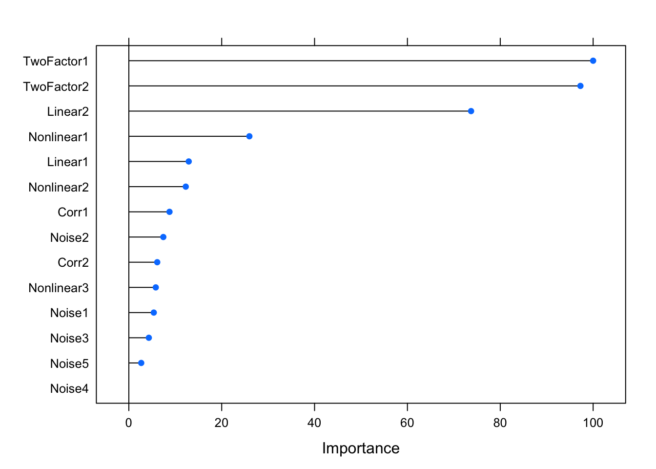
Let’s fit a couple of other models before moving on. One common choice would be the elastic net. Elastic net relies on L1 and L2 regularisations and it’s basically a mix of both: the former shrinks some variable coefficients to zero (so that they are dropped out; i.e. feature selection/dimensionality reduction), whereas the latter penalises coefficient size. In R, it has two hyper-parameters that can be tuned: alpha and lambda. Alpha controls the type of regression; 0 representing Ridge and 1 denoting LASSO (Least Absolute Shrinkage and Selector Operator)2. Lambda, on the other hand, determines the penalty amount. Note that the expand.grid function actually just creates a dataset with two columns called alpha and lambda, which are then used for the model fit based on the value-pairs in each row.
set.seed(1895)
glmnet.fit <- train(x = predictors, y = y, trControl = cls.ctrl,
                    method = "glmnet", metric = "ROC",
                    preProcess = c("nzv", "center", "scale"),
                    tuneGrid = expand.grid(alpha = 0:1,
                                           lambda = seq(0.0001, 1, length = 20)))
Because it has tune-able parameters, we can visualise their performance by calling plot on the model fit:
plot(glmnet.fit)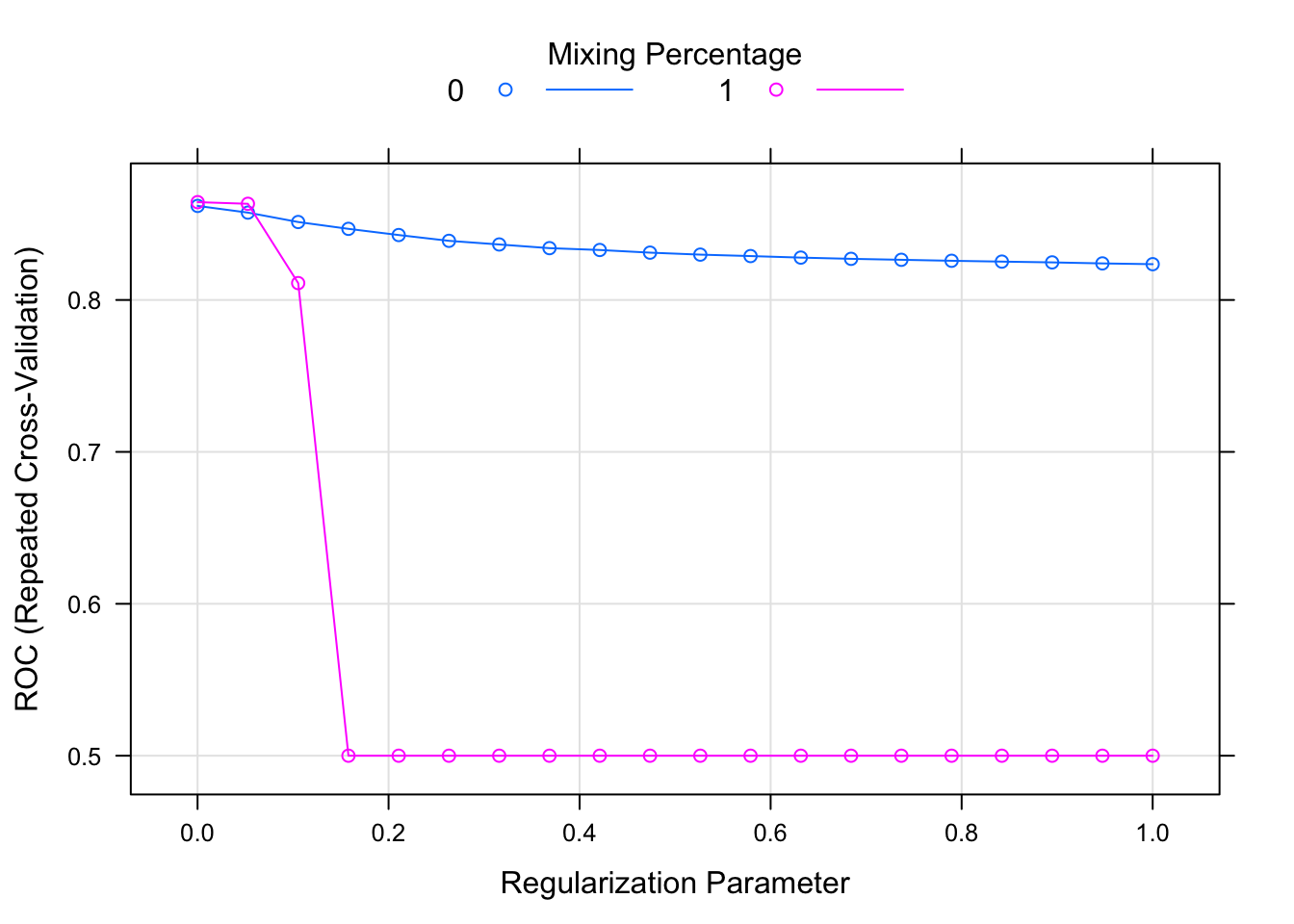
where the two colours denote the alpha level and the dots are the specified lambda values.
Finally, let’s fit a Random Forest using the ranger package, which is a fast C++ implementation of the original algorithm in R:
set.seed(1895)
rf.fit <- train(Class ~ ., data = training, trControl = cls.ctrl,
                method = "ranger", metric = "ROC",
                preProcess = c("nzv", "center", "scale"))
confusionMatrix(rf.fit)
## Cross-Validated (10 fold, repeated 5 times) Confusion Matrix
##
## (entries are percentual average cell counts across resamples)
##
## Reference
## Prediction Class1 Class2
## Class1 51.2 7.2
## Class2 5.4 36.1
##
## Accuracy (average) : 0.8739This is all good, as we are fitting different algorithms using a simple interface without needing to memorise the idiosyncrasies of each package. However, we are still writing lots of redundant code. The caretEnsemble package provides this functionality via caretList:
set.seed(1895)
models <- caretList(Class ~ ., data = training, trControl = cls.ctrl, metric = "ROC",
                    tuneList = list(logit = caretModelSpec(method = "glm", family = "binomial"),
                                    elasticnet = caretModelSpec(method = "glmnet",
                                                                tuneGrid = expand.grid(alpha = 0:1,
                                                                                       lambda = seq(0.0001, 1, length = 20))),
                                    rf = caretModelSpec(method = "ranger")),
                    preProcess = c("nzv", "center", "scale"))
We basically just merged the first three model fits into a single call using tuneList, which requires a list of model specifications. If we want to predict using unseen data, we can now get predictions from all three models:
models.preds <- lapply(models, predict, newdata = test) #add type = "prob" for class probabilities
models.preds <- data.frame(models.preds)
head(models.preds, 10)
## logit elasticnet rf
## 1 Class1 Class1 Class1
## 2 Class2 Class2 Class2
## 3 Class1 Class1 Class2
## 4 Class2 Class2 Class1
## 5 Class1 Class1 Class2
## 6 Class2 Class2 Class2
## 7 Class2 Class2 Class2
## 8 Class1 Class1 Class2
## 9 Class1 Class1 Class1
## 10 Class1 Class1 Class1The resamples function collects all the resampling data from all models and allows you to easily assess in-sample performance metrics:
bwplot(resamples(models)) #try dotplot as well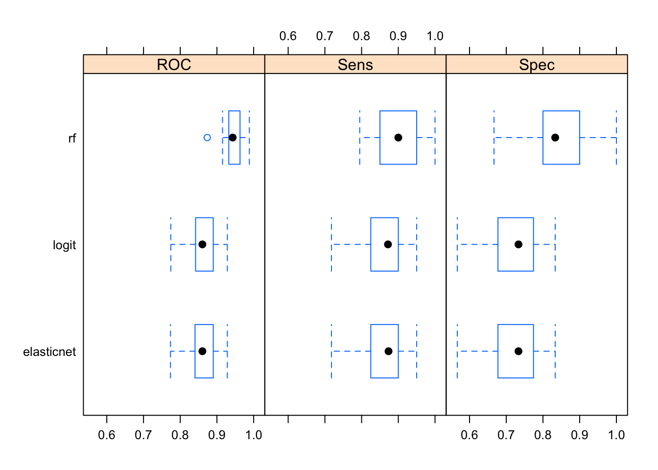
Averaged over all resamples, the Random Forest algorithm has the highest ROC value, however the whiskers overlap in all three categories—perhaps a larger number of resamples are needed for significant separation. It also outperforms other two algorithms when it comes to detecting true positives and true negatives. Note that often the results will not be this clear; it’s common for an algorithm to do really well in one area and perform terribly in the other.
We could also create a simple linear ensemble using the three model fits. You can check whether the model predictions are linearly correlated:
modelCor(resamples(models))## logit elasticnet rf
## logit 1.0000000 0.9996123 0.1135033
## elasticnet 0.9996123 1.0000000 0.1141322
## rf 0.1135033 0.1141322 1.0000000Seems like logit and elastic net predictions are more or less identical, meaning one of them is redundant:
xyplot(resamples(models))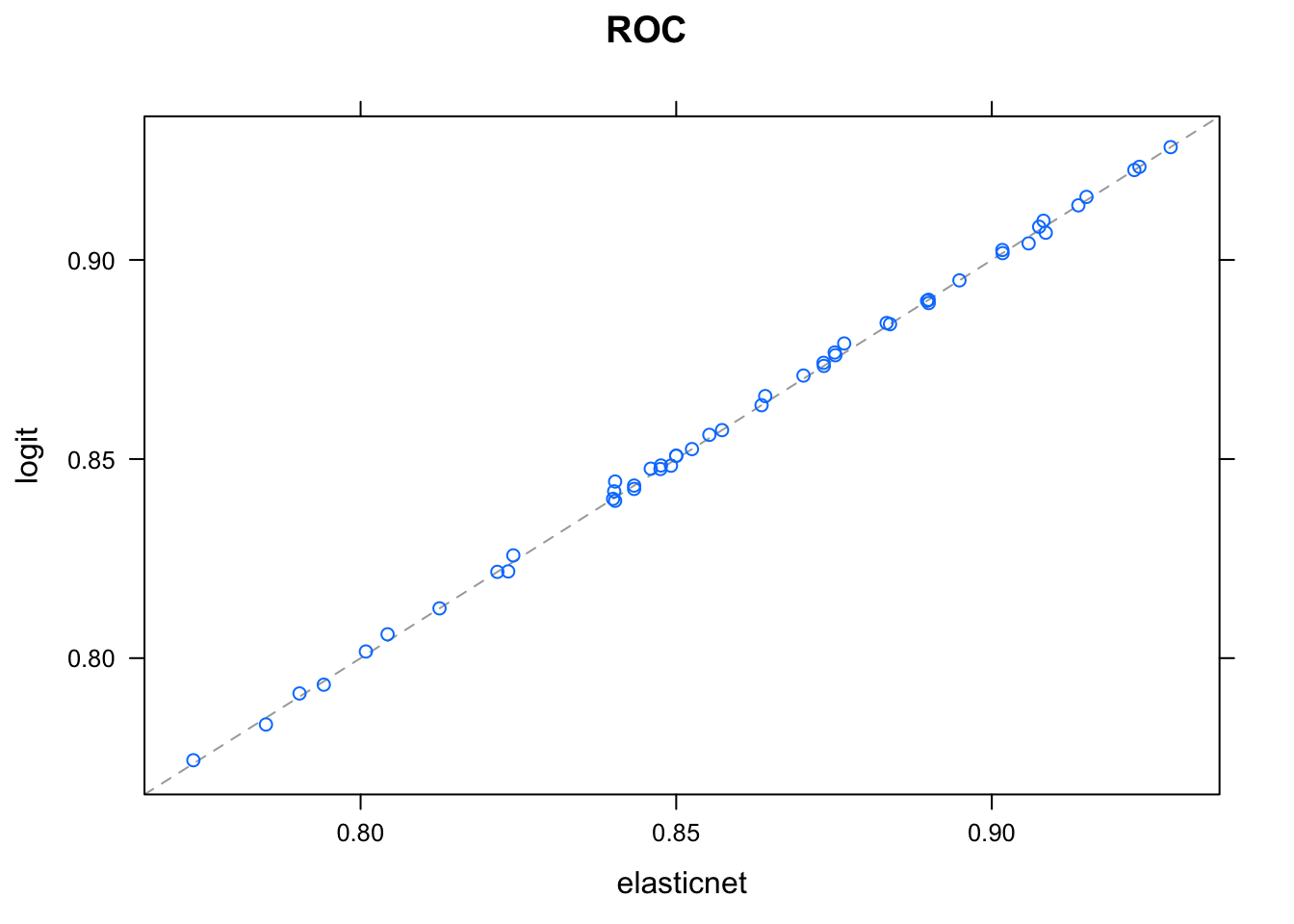
And now for the ensemble:
set.seed(1895)
greedy_ensemble <- caretEnsemble(models, metric = "ROC", trControl = cls.ctrl)
summary(greedy_ensemble)
## The following models were ensembled: logit, elasticnet, rf
## They were weighted:
## -4.9237 44.2633 -42.2176 8.0329
## The resulting ROC is: 0.9517
## The fit for each individual model on the ROC is:
## method ROC ROCSD
## logit 0.8618236 0.03919733
## elasticnet 0.8614454 0.03923875
## rf 0.9469568 0.02237265The ROC of the ensemble (0.9517) is higher than any individual model, however the Random Forest algorithm by itself provides similar levels of accuracy (0.9469).
Feature Selection
As an extra, I’ll briefly cover several feature selection wrapper functions that are available in caret.
Recursive Feature Elimination
RFE works by passing a vector of subsets consisting of different number of variables to be used in model fitting. For example, because we only have 14 variables in our dataset (excluding the outcome), we can try all numbers from one to 14. With all three feature selection algorithms, we will need to change the summary function to twoClassSummary for classification purposes.
subsets <- c(1:length(training))

lrFuncs$summary <- twoClassSummary
We need to pass an additional control function specifically for the RFE. We select the linear regression wrapper (lrFuncs),3 and choose bootstrapped cross-validation (25). After that, we call the rfe function:
rfe.ctrl = rfeControl(functions = lrFuncs,
                      method = "boot",
                      number = 25,
                      allowParallel = TRUE, verbose = TRUE)

set.seed(1895)
rfe <- rfe(x = predictors, y = y, sizes = subsets,
           metric = "ROC", rfeControl = rfe.ctrl)
rfe
##
## Recursive feature selection
##
## Outer resampling method: Bootstrapped (25 reps)
##
## Resampling performance over subset size:
##
## Variables ROC Sens Spec ROCSD SensSD SpecSD Selected
## 1 0.6383 0.8529 0.4462 0.03546 0.03912 0.05763
## 2 0.8123 0.8351 0.6355 0.03603 0.04063 0.04609
## 3 0.8606 0.8723 0.6905 0.01693 0.03575 0.04339
## 4 0.8610 0.8634 0.6958 0.01955 0.03571 0.04740 *
## 5 0.8596 0.8595 0.7011 0.01893 0.03560 0.04360
## 6 0.8582 0.8574 0.7010 0.01925 0.03567 0.04386
## 7 0.8565 0.8565 0.6983 0.01996 0.03595 0.04805
## 8 0.8565 0.8557 0.7017 0.01907 0.03565 0.04726
## 9 0.8561 0.8590 0.6993 0.01988 0.03484 0.04806
## 10 0.8560 0.8569 0.7052 0.02019 0.03384 0.04739
## 11 0.8560 0.8592 0.7048 0.02003 0.03353 0.04939
## 12 0.8561 0.8558 0.7047 0.02014 0.03430 0.04612
## 13 0.8561 0.8561 0.7051 0.02015 0.03413 0.04721
## 14 0.8562 0.8555 0.7047 0.01999 0.03407 0.04688
##
## The top 4 variables (out of 4):
## TwoFactor1, TwoFactor2, Linear2, Nonlinear1We see that the model with four variables (indicated with an asterisk) resulted in the highest ROC value and thus selected as the best model. The top variables are also displayed at the end. One approach would be fitting a model on the test data using these four variables only.
Simulated Annealing
SA works by starting with a certain number of variables and introducing small changes to them along the way. If the change results in an `upgrade’ (i.e. higher predictive accuracy), the initial candidate is abandoned in favour of the new solution. Unlike RFE, which is greedy—meaning, it only assesses the subset sizes once and moves on forever—SA can be programmed to go back and try again if it doesn’t find an improvement within a certain number of iterations (below we set this limit to 5). We can also pass which performance metrics to be used for both the internal and external processes, as well as defining the amount that will be held out (20%):
caretSA$fitness_extern <- twoClassSummary

safs.ctrl = safsControl(functions = caretSA, method = "boot", number = 10,
                        metric = c(internal = "ROC", external = "ROC"),
                        maximize = c(internal = TRUE, external = TRUE),
                        holdout = .2, improve = 5,
                        allowParallel = TRUE, verbose = TRUE)
We can then fit the algorithm by calling safs:
sa <- safs(x = predictors, y = y,
           iters = 10, method = "glm", family = "binomial", metric = "ROC",
           trControl = cls.ctrl,
           safsControl = safs.ctrl)
## + final SA
## 1 0.4597138 (3)
## 2 0.4597138->0.4663124 (3+1, 75.0%) *
## 3 0.4663124->0.4626936 (4-1, 75.0%) 0.9769874 A
## 4 0.4663124->0.6563141 (4+0, 60.0%) *
## 5 0.6563141->0.657809 (4-1, 75.0%) *
## 6 0.657809->0.7425797 (3+1, 75.0%) *
## 7 0.7425797->0.7398033 (4+1, 80.0%) 0.9741674 A
## 8 0.7425797->0.7417647 (4+0, 60.0%) 0.991258 A
## 9 0.7425797->0.7407108 (4+1, 50.0%) 0.9776039 A
## 10 0.7425797->0.7427323 (4+0, 60.0%) *
## + final modelCalling the object returns an informative summary of the whole process:
sa##
## Simulated Annealing Feature Selection
##
## 701 samples
## 14 predictors
## 2 classes: 'Class1', 'Class2'
##
## Maximum search iterations: 10
## Restart after 5 iterations without improvement (0.3 restarts on average)
##
## Internal performance values: ROC, Sens, Spec
## Subset selection driven to maximize internal ROC
##
## External performance values: ROC, Sens, Spec
## Best iteration chose by maximizing external ROC
## External resampling method: Bootstrapped (10 reps)
## Subsampling for internal fitness calculation: 20%
##
## During resampling:
## * the top 5 selected variables (out of a possible 14):
## Linear2 (70%), TwoFactor1 (70%), TwoFactor2 (70%), Nonlinear1 (60%), Corr1 (40%)
## * on average, 5.6 variables were selected (min = 3, max = 8)
##
## In the final search using the entire training set:
## * 4 features selected at iteration 10 including:
## TwoFactor1, Linear2, Noise3, Noise4
## * external performance at this iteration is
##
## ROC Sens Spec
## 0.7539 0.8022 0.5891Genetic Algorithm
Last but not least, we will cover genetic algorithms. Here, variables are put through pressures similar to that of natural selection. We keep the iteration and population sizes really, really low as the code chunks are only supposed to give you a working example of the process. These algorithms fit a lot of models, so always start with a small value and gradually increase the number of iterations/generations.
caretGA$fitness_extern <- twoClassSummary

gafs.ctrl = gafsControl(functions = caretGA, method = "boot", number = 10,
                        metric = c(internal = "ROC", external = "ROC"),
                        maximize = c(internal = TRUE, external = TRUE),
                        holdout = .2,
                        allowParallel = TRUE, genParallel = TRUE, verbose = TRUE)

set.seed(1895)
ga <- gafs(x = predictors, y = y, iters = 5, popSize = 2, elite = 0,
           differences = TRUE, method = "glm", family = "binomial", metric = "ROC",
           trControl = cls.ctrl,
           gafsControl = gafs.ctrl)
## + final GA
## 1 0.8197197 (12)
## 2 0.8197197->0.820586 (12->12, 100.0%) *
## 3 0.820586->0.8211813 (12->12, 100.0%) *
## 4 0.8211813->0.8218709 (12->12, 100.0%) *
## 5 0.8218709->0.8215376 (12->12, 100.0%)
## + final modelSimilar to the previous algorithms, calling the final object provides a summary:
ga##
## Genetic Algorithm Feature Selection
##
## 701 samples
## 14 predictors
## 2 classes: 'Class1', 'Class2'
##
## Maximum generations: 5
## Population per generation: 2
## Crossover probability: 0.8
## Mutation probability: 0.1
## Elitism: 0
##
## Internal performance values: ROC, Sens, Spec
## Subset selection driven to maximize internal ROC
##
## External performance values: ROC, Sens, Spec
## Best iteration chose by maximizing external ROC
## External resampling method: Bootstrapped (10 reps)
## Subsampling for internal fitness calculation: 20%
##
## During resampling:
## * the top 5 selected variables (out of a possible 14):
## Linear2 (100%), Noise3 (100%), Nonlinear3 (100%), TwoFactor2 (100%), Corr2 (90%)
## * on average, 12.4 variables were selected (min = 10, max = 14)
##
## In the final search using the entire training set:
## * 12 features selected at iteration 1 including:
## TwoFactor1, TwoFactor2, Linear1, Nonlinear1, Nonlinear2 ...
## * external performance at this iteration is
##
## ROC Sens Spec
## 0.8475 0.8481 0.7055Given the small number of iterations used for SA and GA, we can’t really judge the quality of their results. However, running the algorithms for hundreds or thousands of iterations is not necessarily the best option either. As these algorithms focus on maximising in-sample ROC, given enough iterations, they will perfectly learn the specific noise of your dataset and will not generalise to unseen data (i.e. over-fitting). As always, aim to leverage your domain knowledge and gradually increase the number of iterations until you see a divergence between training and test validation results.
Big fan of coming up with original names.↩
Seriously, who names these things? Backronyms everywhere.↩